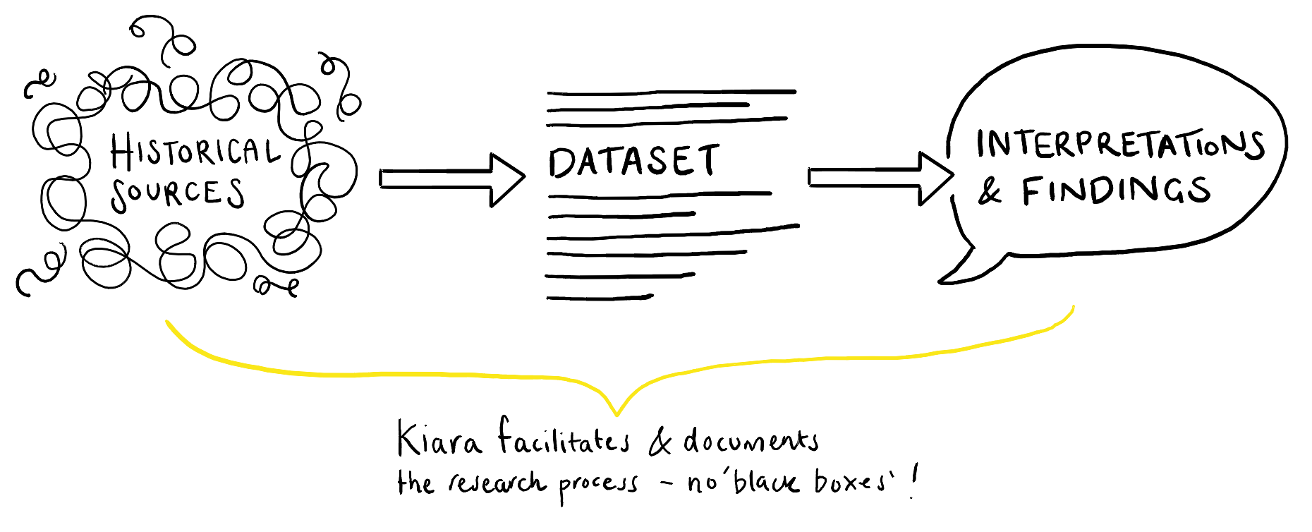
# What is kiara?
*Kiara* is a **data orchestration tool** designed for digital humanities researchers who want to maintain a critically aware relationship with their sources and data. Developed by the **DHARPA project** (Digital History Advanced Research Projects Accelerator) at the Luxembourg Centre for Contemporary and Digital History, kiara addresses a fundamental challenge in digital humanities: how to preserve scholarly agency and critical engagement when using computational methods.
Unlike conventional data processing tools that often function as "black boxes," kiara is built to illuminate the research process from start to finish. It's a **Python-based** tool that combines the technical power of data [pipeline](/before-you-begin/key-concepts#pipeline) frameworks with a strong emphasis on transparency, documentation, and critical reflection.
At its core, kiara is **modular and data-centric**, allowing researchers to document their engagement with sources at every step through [lineages](/before-you-begin/key-concepts#lineage) of their [workflow](/before-you-begin/key-concepts#workflow). Whether you're analyzing texts, building network graphs, or processing historical data, kiara helps you maintain awareness of how your sources are transformed into computer-legible data and how your methodological choices shape your research outcomes.
The tool operates via command line or Jupyter notebooks, making it accessible to researchers with basic Python familiarity while offering the depth and flexibility needed for advanced digital humanities projects. By developing additional [plugins](/before-you-begin/key-concepts#plugin), more competent users can extend and customise kiara.
# What can kiara do?
Kiara enables digital humanities researchers to:
* **Create and customize data workflows**: Use pre-built modules for common DH tasks in network analysis and topic modeling, or adapt existing Python code into new modular components that can be rearranged and chained together according to your specific research needs.
* **Document the research process with comprehensive metadata**: Automatically track and record all transformations your data undergoes, creating a complete data lineage with both automatic and manual metadata. This documentation enables critical reflection on your methodological choices and supports writing a self-reflexive meta-history of your relationship with your sources.
* **Make informed methodological decisions**: Each module provides clear descriptions of the required inputs and expected outputs, helping you understand what's happening at each step and make conscious choices about how to proceed.
* **Interactive exploration with accountability**: Unlike most batch processing tools, kiara offers an interactive approach that allows you to engage with your data at crucial decision points while still maintaining a record of your actions and choices.
* **Share and collaborate**: Create modular components that can be shared with other researchers, enabling collaborative development of digital humanities methodologies.
Kiara particularly excels at the preparation, transformation, and initial analysis stages of research, providing fine-grained control over processes that are often hidden inside "black box" tools. By encouraging transparency and traceability, it helps researchers maintain and share their critical thinking as they leverage computational methods.
# What is data orchestration?
Data orchestration is the process of managing and conducting data-related tasks. In kiara, you can organize, transform, and track your research data throughout the analytical process.
### From Sources to Data
Historical sources don't arrive as neatly structured data. Letters, census records, newspapers, and other primary sources must be transformed into machine-readable formats before computational analysis becomes possible. This transformation process, in which you *create* your dataset, involves critical decisions that shape your research outcomes – yet many digital tools obscure that process. When you simply click through software interfaces, you may lose sight of how your sources become data, how that data is manipulated, and ultimately how your interpretations relate to the original materials.
### Data Orchestration, documented
Kiara therefore allows you to both perform and track each of those steps. Rather than processing your data through monolithic "black box" tools, kiara facilitates the creation of data [pipelines](/before-you-begin/key-concepts#pipeline) that consist of distinct, interconnected [modules](/before-you-begin/key-concepts#module). Each module has clearly defined inputs, outputs, and processes, allowing you to understand exactly what is happening to your data at each step. At the same time, kiara automatically tracks the ancestry of your data through every transformation. At any point, you can see the [lineage](/before-you-begin/key-concepts#lineage) of how a particular dataset was created, including all the inputs and processes involved, making your [workflow](/before-you-begin/key-concepts#workflow) and findings both explainable and reproducible.
# Key concepts
Understanding these core concepts will help you work effectively with kiara:
## Module
A module is kiara's basic building block for data operations. Each module is a self-contained unit designed to perform a specific task within your research workflow. A kiara module consists of three essential sections:
* **Input**: Specifies what data the module requires, with descriptions of expected properties to help you make informed decisions.
* **Process**: Contains the Python code required to execute the module.
* **Output**: Defines what the module will produce after processing.
For example, the `` module requires three inputs: a graph object, a nodes table, and a string (the column name for node indexes), and outputs an augmented graph object. The user can find out what the necessary inputs are at any time by using the command:
```
kiara operation explain [insert module name]
```
Partial view of Kiara's explanation of the assemble.network_graph module
## Plugin
A plugin in kiara is a collection of related modules that extend the system's functionality. Plugins allow researchers to add specialized capabilities without modifying the core system. Anyone with basic Python knowledge can create plugins by adapting existing Python code into kiara's module structure, making the system highly extensible and community-driven.
## Pipeline
A pipeline is a sequence of connected modules where the output of one module becomes the input for another. Kiara's modular approach allows you to create pipelines that compartmentalize workflow steps that would typically appear in a single Python script. This compartmentalization enables greater flexibility, as modules can be rearranged and recombined to create different analytical pathways according to your research needs.
## Workflow
A workflow in kiara represents your entire research process, potentially consisting of multiple pipelines and individual modules. Workflows can be saved, shared, reused, and modified. The workflow concept is central to kiara's approach to transparency and reproducibility, as it captures not just individual operations but the entire sequence of transformations your data undergoes during research.
## Lineage
Lineage (or data ancestry) is kiara's record of how data values are created and transformed throughout your research process. When you request the lineage of a data object (using a command like ``), kiara provides a comprehensive history showing all the modules and inputs that contributed to creating that object.
For example, requesting the lineage of a network graph might show that it was first created from an edges table and later augmented with additional node attributes from a separate data source. This lineage documentation is crucial for understanding data provenance, ensuring research transparency, and enabling critical reflection on methodological choices.
Kiara lineage visualisation
## Context
Kiara has a default context which is always available, but users can also create different contexts within their virtual environment for each project they undertake with kiara. Each context stores:
* the data you import or create
* the operations you run
* your notes and decisions
# Mac
How to install kiara and its dependencies in a virtual environment for Mac users
### Prerequisites
If you haven't already, install the latest versions of:
* [miniconda](https://www.anaconda.com/docs/getting-started/miniconda/main) (a tool for managing Python and dependencies)
* [Git](https://git-scm.com/book/en/v2/Getting-Started-Installing-Git) (a version control system)
> Tip: We recommend using Homebrew or another package manager for installing these.
### Creating and activating an environment
Open a new Terminal window and create an environment to install kiara into. This is like giving kiara its own room, so that it will not interfere with other tools or projects on your computer. For example:
```⏎
conda create -n kiara_explore
```
You can replace `kiara_explore` with any name you choose for your environment.
Proceed by typing `y` and hitting enter, before activating the conda environment using:
```⏎
conda activate kiara_explore
```
### Install kiara and its basic plugins
Kiara is installed using a package-management system for Python called `pip`. To install pip into your environment, use:
```
conda install pip
```
Then:
```⏎
pip install kiara
```
The installation may take a few minutes. Once complete, install kiara's plugins:
```
pip install kiara_plugin.core_types kiara_plugin.onboarding kiara_plugin.tabular
```
These plugins provide support for:
* core data types
* helpful onboarding tools
* tabular data (spreadsheets, CSVs, etc.)
> Tip: to check which version of kiara or any of its plugins are installed at any point, use `pip list | grep kiara`
Example output for pip list | grep kiara
# Windows
How to install kiara and its dependencies in a virtual environment for Windows users
### Prerequisites
If you haven't already, install the latest versions of:
* [miniconda](https://www.anaconda.com/docs/getting-started/miniconda/main) (a tool for managing Python and dependencies)
* [Git](https://git-scm.com/book/en/v2/Getting-Started-Installing-Git) (a version control system)
> Tip: Package managers like Chocolatey or Scoop can be used instead of manual downloads.
### Creating and activating an environment
Open your Command Line Interface and create an environment to install kiara into. This is like giving kiara its own room, so that it will not interfere with other tools or projects on your computer. For example:
```⏎
conda create -n kiara_explore
```
You can replace `kiara_explore` with any name you choose for your environment.
Activate the conda environment:
```⏎
conda activate kiara_explore
```
### Install kiara and its basic plugins
Kiara is installed using a package-management system for Python called `pip`. Simply use:
```⏎
pip install kiara
```
The installation may take a few minutes. Once complete, install kiara's plugins:
```
pip install kiara_plugin.core_types kiara_plugin.onboarding kiara_plugin.tabular
```
These plugins provide support for:
* core data types
* helpful onboarding tools
* tabular data (spreadsheets, CSVs, etc.)
> Tip: to check which version of *kiara* or any of its plugins are installed at any point, use `pip list | findstr kiara`
# Basic data processing in Jupyter
## Activate your kiara environment
As you have seen in the install instructions, you need to create a special [environment](https://docs.anaconda.com/working-with-conda/environments/) for kiara to run in. Use the following command to activate your previously created kiara environment, replacing `kiara_explore` with whatever name you assigned it:
```
conda activate kiara_explore
```
> Tip: to check what environments you have created in the past, you can use `conda env list`
## Dependencies
You already installed some basic plugins when setting up your kiara environment. Now you can use conda to also install the necessary packages for using kiara in Jupyter notebooks.
You'll be using Jupyter notebook and Observable within that notebook, so enter:
```
conda install jupyter observable_jupyter
```
## Start Jupyter notebook
To open the Jupyter interface, run:
```
jupyter notebook
```
## Import kiara and create an API
Open a new notebook using the option on the top right of the Jupyter interface. Now, to start using kiara in Jupyter Notebook, you first need to create a `kiaraAPI` **instance**. This instance allows us to control kiara and see what operations are available.
To set this up, run the following code in a notebook cell:
```
from kiara.api import KiaraAPI
kiara = KiaraAPI.instance()
```
## Create a project context
In kiara, a [**context**](/before-you-begin/key-concepts#context) is your project space. To create and use a **new context** called `project1_DP`, run the following code:
```
kiara.set_active_context(context_name='project1_DP', create=True)
print('Available Contexts:', kiara.list_context_names())
print('Current Context:', kiara.get_current_context_name())
```
This operation will also show all your available contexts and confirm which one is currently active. The output will be something like:
```
Available Contexts: ['default', 'project1_DP']
Current Context: project1_DP
```
This confirms that your new context is set up and ready to use.
## Explore kiara operations
Now, you can explore the tools kiara offers. To view a list of all available **operations** (based on the installed plugins), run:
```
kiara.list_operation_ids()
```
This will return a list of operations:
Partial view of the returned operations list
Each **operation** is a task you can perform in kiara, such as creating a table, calculating network metrics, or exporting files.
## Download a file
Now that kiara is set up, let's bring a file into your notebook using the `download.file` operation.
To understand what this operation does and what information it needs, run:
```
kiara.retrieve_operation_info('download.file')
```
You will now download a sample CSV file using this operation. First, you define the **input** (the file URL and name) and then run the job:
```
inputs = {
"url": "https://raw.githubusercontent.com/DHARPA-Project/kiara.examples/main/examples/data/network_analysis/journals/JournalNodes1902.csv",
"file_name": "JournalNodes1902.csv"
}
outputs = kiara.run_job('download.file', inputs=inputs, comment="importing journal nodes")
```
This gives you a **file object** as **output**, including the downloaded file and some technical metadata. Let’s print it to confirm:
```
outputs
```
You will see a preview of the file's content. This shows the journal data was successfully downloaded.
## Save the downloaded file
To keep using this file later (even if the notebook is closed), you will save it inside kiara using an **alias**. This works like giving a name that kiara remembers.
```
downloaded_file = outputs['file']
kiara.store_value(value=downloaded_file.value_id, alias='Journal_Nodes')
```
Now, `Journal_Nodes` is saved in kiara's internal storage. You can refer to it later just by its alias.
## Convert the file into a table
Now that you have downloaded the file, let's turn it into a **table** so you can work with the data.
You can look through kiara’s available operations by filtering for those that start with `create`:
```
kiara.list_operation_ids('create')
```
This shows a list of operations. Since you are working with a CSV file, the one you want is `create.table.from.file` .
This operation will read the file and turn it into a **structured table**.
To see what inputs and outputs this operation expects, run:
```
op_id = 'create.table.from.file'
kiara.retrieve_operation_info(op_id)
```
From this, you learn the inputs and outputs:
**Inputs**
* Required: a file.
* Optional:
* `first_row_is_header` – indicates if the first row of a CSV file contains column headers.
* `delimiter` – specifies the column separator (only for CSV), used if kiara cannot auto-detect it.
**Outputs**
* A `table` object, which can be used in the next steps.
Let’s turn the downloaded file (which you saved earlier under the alias `Journal_Nodes`) into a **table**:
```
inputs = {
"file": kiara.get_value('Journal_Nodes'),
"first_row_is_header": True
}
outputs = kiara.run_job(op_id, inputs=inputs, comment="")
outputs
```
This will process the CSV file and show the result as a **table** with **columns** and **rows**.
## Save the table
To make it easier to reuse the table later, you can save it in kiara under a **new alias**:
```
outputs_table = outputs['table']
kiara.store_value(value=outputs_table.value_id, alias="Journal_Nodes_table")
```
Now, your data is saved inside kiara and can be accessed at any time using the name `Journal_Nodes_table`.
## Query the data
Now that you have downloaded the file and converted it into a table, you can start exploring the data. One simple way to do that is by running **SQL queries** directly on the table using κiara.
To find relevant operations for querying data, search with the keyword `'query'`:
```
kiara.list_operation_ids('query')
```
This returns:
```
['query.database', 'query.table']
```
Since you are working with a table, you will use:
```
kiara.retrieve_operation_info('query.table')
```
This tells us that `query.table` allows us to write an **SQL query** to explore the data.
The required **inputs** are:
* `table`: the data you want to query
* `query`: your SQL statement
Let’s find out how many of these journals were published in Berlin:
```
inputs = {
"table": kiara.get_value('Journal_Nodes_table'),
"query": "SELECT * from data where City like 'Berlin'"
}
outputs = kiara.run_job('query.table', inputs=inputs, comment="")
outputs
```
The result (in `outputs['query_result']`) is a filtered table showing only journals published in Berlin.
## Refine the query
Let's narrow this further and find all the journals that are about general medicine and published in Berlin.
You can re-use the `query.table` function and the table you have just made, stored in `outputs['query_result']`
```
inputs = {
"table" : outputs['query_result'],
"query" : "SELECT * from data where JournalType like 'general medicine'"
}
outputs = kiara.run_job('query.table', inputs=inputs, comment="")
outputs
```
This returns a smaller table with only the Berlin-based general medicine journals.
## Record and trace your data
Now that you have transformed and queried your data, let's review what κiara knows about the outputs you have created and how it tracks changes. **Data lineage** is one of kiara’s most powerful features.
Let’s check the lineage of your query output:
```
query_output = outputs['query_result']
query_output
```
Even though you have made changes along the way, you can still access a lot of information about your data.
kiara automatically traces all of these changes, **keeping track of** **inputs** and **outputs** and assigning each a unique identifier, so you always know exactly what has happened to your data.
To have a 'backstage' view of how your data was transformed, including the inputs for each function you have run and how they connect, run the following:
```
query_output.lineage
```
Each input is assigned a unique ID, allowing complete transparency and traceability.
You can also **visualize** the lineage by running:
```
lineage = kiara.retrieve_augmented_value_lineage(query_output)
from observable_jupyter import embed
embed('@dharpa-project/kiara-data-lineage', cells=['displayViz', 'style'], inputs={'dataset':lineage})
```
## Review and export all jobs
kiara keeps a **record** of all operations you’ve run in this context.
You can print out this history:
```
kiara.print_all_jobs_info_data(show_inputs=True, show_outputs=True, max_char=100)
```
Finally, you can **export** your job log to a CSV file to keep a full record of what you’ve done:
```
import pandas as pd
job_table = pd.DataFrame(kiara.get_all_jobs_info_data(add_inputs_preview=True, add_outputs_preview=True))
job_table.to_csv('job_log.csv', index=False)
```
# Network analysis in Jupyter
## Network analysis with kiara
Now that you are comfortable with what kiara looks like and what it can do to help track your data and your research process, let's try out some of the digital analysis tools, starting with **network analysis**.
## Why network analysis?
Network analysis offers a computational and quantitative means to examine and explore **relational objects**, with proxies to **measure** structural roles and concepts such as power and influence.
Doing this digitally, and **at scale**, enables you to ask questions of large datasets that would be impossible to answer qualitatively.
This tutorial is not a deep dive into network theory or its applications in the humanities. Rather, you will focus on how using kiara helps you structure your workflow, document your decisions, and trace the transformations your data undergoes during analysis.
## Activate your kiara environment
As you have seen in the install instructions, you need to create a special environment for kiara to run in. Using a new CLI window, type the following to activate your previously created kiara environment (replacing `kiara_explore` with whatever name you assigned it):
```
conda activate kiara_explore
```
> Tip: to check what environments you have created in the past, you can use `conda env list`
## Dependencies
You already installed some basic plugins when setting up your kiara environment, and you installed Jupyter notebook and Observable when completing [Basic data processing in Jupyter](/using-kiara/basic-data-processing-in-jupyter). Now you should install the necessary packages for network analysis, too.
You'll be using networkx, so enter:
```
conda install networkx
```
> Tip: to check what packages are already installed in your environment, use `conda list`
## Open Jupyter notebook and set up the kiaraAPI
To open the Jupyter interface, run:
```
jupyter notebook
```
Now we need to set up the `kiaraAPI`, the interface that allows us to run kiara commands inside your Jupyter notebook.
Here is the code to get started:
```
import networkx as nx
import os
from kiara.api import KiaraAPI
kiara = KiaraAPI.instance()
```
## Create a project context
As you saw in the [previous section](/using-kiara/basic-data-processing-in-jupyter), kiara uses different [**contexts**](/before-you-begin/key-concepts#context) for specific projects. To create and use a **new context** for your network analysis project, e.g. `project2_NA,` run the following code:
```
kiara.set_active_context(context_name='project2_NA', create=True)
print('Available Contexts:', kiara.list_context_names())
print('Current Context:', kiara.get_current_context_name())
```
This operation will also show all your available contexts and confirm which one is currently active. The output will be something like:
```
Available Contexts: ['default', 'project1_DP', 'project2_NA']
Current Context: project2_NA
```
This confirms that your new context is set up and ready to use.
## Set up your data path
Next, you need to set the **file path** to the data you will use in this notebook.
In this example, the CSV file is stored in the same directory as the notebook, inside a subfolder named `data`.
You can either write out the full file path, or use Python's `os.path` module to construct it, as below:
```
notebook_path = os.path.abspath('')
csv_file_path = os.path.join(notebook_path,"data/CKCC.csv")
```
## About the dataset
The dataset you are working with comes from the *Circulation of Knowledge and Learned Practices in the 17th-century Dutch Republic (CKCC)* collection.
This corpus of around 20,000 letters exchanged between scholars in the Dutch Republic during the 17th century. It was compiled by the Huygens Institute in the Netherlands and is available through the LetterSampo portal as part of the *Reassembling the Republic of Letters* project.
By applying network analysis, you can explore questions such as:
* Who was the most prolific writer?
* Which actor connected the most people?
* Who operated in closely knit writing groups?
Although network analysis can be used to explore unfamiliar datasets, in this case, you already have some prior knowledge of the material. The research questions and parameter choices in this notebook reflect that prior knowledge — something to keep in mind as you proceed.
## Import data
Now you will import the data using kiara's `import.local.file` operation.
This module allows you to import any local file - in this case, your CSV file. You are using a sample dataset here, but you can also use this same module to import your own data.
You will pass the file path you defined earlier as an input. You will also save the output of this operation under the alias 'CKCC'. Alternatively, you can use the `download.file` module mentioned above.
You can leave the `comment` field empty for now — or you might use it to note why you chose this dataset, or which version you are working with (if you have multiple versions of the same data).
Here is the code:
```
CKCC = kiara.run_job('import.local.file', inputs={'path': csv_file_path}, comment="importing bits")
```
## Create a network
Now that you have imported your data, it’s time to build a **network** from it.
To create a network, kiara expects your data to be in the form of an **edge table**. An edge table lists relationships between entities — in this case, between senders and recipients of letters. Later, you could also add a **node table** (a table listing all the individual entities), but this is optional — you will skip it for now.
## Convert your CSV into an edge table
To turn your CSV file into an edge table, you will use the `create.table.from.file` function that you used earlier.
You will first check what inputs this function requires:
```
kiara.retrieve_operation_info('create.table.from.file')
```
This will display helpful information about what inputs the function expects and what it returns.
Now, you can load your CSV data (which you imported earlier and stored in `CKCC`) and tell kiara that the first row contains column headers:
```
inputs = {
"file": CKCC['file'],
"first_row_is_header": True
}
outputs = kiara.run_job('create.table.from.file', inputs=inputs, comment="")
edges = outputs['table']
outputs
```
At this point, you have created your **edges table**, which will serve as the basis for your network graph.
## Preview the network structure
Before you assemble your network graph, it is helpful to preview its structure.
You can do this using kiara’s `preview.network_info` function.
This function will show you:
* How many nodes and edges the network contains
* How the graph structure might change depending on whether you choose **directed**, **undirected**, **multi-directed**, or **multi-undirected** representations
To run the preview, specify your edges table, along with the source and target columns:
```
inputs = {'edges': edges,
'source_column': 'Source',
'target_column': 'Target'}
network_info = kiara.run_job('preview.network_info', inputs=inputs, comment="")
network_info
```
This preview will give you useful insights:
* If there are more edges in a **directed** graph than in an **undirected** one, it suggests that some nodes are reciprocally connected, as is common in letter networks.
* If a **multigraph** has even more edges, this means that **parallel edges** exist between the same pairs of nodes (for example, one person sending several letters to another).
* If there are **no isolates** (nodes without any edges) and several **components**.
* If you see a large number of **self-loops** (nodes connected to themselves), this is unusual in epistolarly collections and could indicate an issue with the data, for example, missing or misformatted recipient information.
This module helps you decide what type of graph is appropriate for your dataset, and also alerts you to any potential data quality issues you may want to address.
In this case, a **directed graph** makes sense, since letters are sent from one person to another.
## Review the assemble network graph module
Next, you will use the `assemble.network_graph` module to actually build your graph.
Before you run it, it’s helpful to check its inputs:
```
kiara.retrieve_operation_info('assemble.network_graph')
```
This is a flexible module that allows you to make several important decisions:
* The **type of graph** you want to create (directed or undirected)
* Whether the graph should be **weighted** or not
* How to handle **parallel edges**
* If you have a **node table**, you can include it — but this is optional
If you later decide to change your mind about how to structure your graph, you can simply re-run this step.
That’s why previewing the network first is so helpful — it gives you the information you need to make an informed decision.
## Assemble the network graph
Now that you have reviewed the structure of your data, you are ready to assemble the graph.
For this dataset, you will create a **directed graph**.
You will also choose to create a **weighted graph**, where the weight of each edge reflects the **number of letters** sent between two people.
If the dataset contains parallel edges (which the preview revealed), you can choose how to aggregate them. In this case, you will choose `'sum'` — which will count how many times each edge occurs.
Keep in mind that if you have not provided any weights in the data, kiara will automatically assign a weight of 1 to each edge. In that case, selecting `mean` , `minimum`, or `maximum` will simply return 1 for every edge, making the result the same as an **unweighted** network.
Here is the full set of inputs:
```
inputs = {
'graph_type': 'directed',
'edges': edges,
'source_column': 'Source',
'target_column': 'Target',
'is_weighted': True,
'parallel_edge_strategy':'sum'
}
CKCC = kiara.run_job('assemble.network_graph', inputs=inputs, comment="")
CKCC
```
Now you have created a kiara **network graph object**.
The output includes both an **edge table** and a **node table**. Since you did not provide a separate node table, kiara automatically extracted node information from the edges.
If you look at the edge table now, you will see that it includes **weights**, calculated based on the number of letters exchanged.
## Extract the largest component
The preview you ran earlier showed that the network has eight **components** (disconnected subgraphs).
You may want to focus your analysis on the **largest component** — the one with the most nodes — since it often contains the most interesting or well-connected part of the network.
You can extract the largest component like this:
```
CKCC_largest_component = kiara.run_job('extract.largest_component', inputs={'network_graph':CKCC['network_graph']}, comment="")
CKCC_largest_component
```
Now you have a new graph containing just the **largest component** of your network, ready for further analysis.
## Structural measures
Now that you have extracted the largest component of your network, you can calculate some basic **structural measures**: the **diameter** and the **average path length**.
These calculations require the graph to be **connected**, which is why it’s important that you are working with the largest component.
## Calculate the diameter
The **diameter** tells you the length of the longest shortest path between any two nodes in the network, in this case, 7 steps.
Here is how you calculate it:
```
diameter = kiara.run_job('calculate.diameter', inputs={'network_component':CKCC_largest_component['largest_component']}, comment='c')
diameter
```
## Calculate the average path length
The **average path length** gives you the average number of steps it takes to get from one node to another, about 2.7 in this case.
Here is how you calculate it:
```
avg_path = kiara.run_job('calculate.average_path', inputs={'network_component':CKCC_largest_component['largest_component']}, comment='c')
avg_path
```
These two metrics give us an idea of the overall structure of the network.
## Statistical measures
Now that you have your network assembled, you can start exploring **centrality measures** — ways of assessing how important or influential each node is in the network.
## Degree centrality
You will start by calculating **degree centrality** using kiara’s `calculate.degree_score` module.
Before running it, check what inputs the module requires:
```
kiara.retrieve_operation_info('calculate.degree_score')
```
Now you can run the calculation:
```
output = kiara.run_job('calculate.degree_score', inputs={'network_graph':CKCC['network_graph']}, comment="")
output
```
This will return a table of **degree scores**:
* **Undirected degree**: number of correspondents
* **Weighted degree**: number of letters sent and received
kiara also adds these degree scores as **node attributes**, so you can use them in later analyses.
## Betweenness centrality
Next, you will calculate **betweenness centrality**.
Again, first check what inputs the module requires:
```
kiara.retrieve_operation_info('calculate.betweenness_score')
```
This module asks you to define whether **weights** should be interpreted as **positive** (indicating strength) or **negative** (indicating distance or cost).
For the epistolary dataset, you will leave this input as `'True'` , as the weight indicates strength (number of letters).
Before running the calculation, save the current network (with degree scores attached):
```
network_graph = output['centrality_network']
```
Now calculate betweenness:
As before, kiara will return a table of **betweenness scores**, and also add these scores to the **node attributes**.
## Eigenvector centrality
You can now calculate **eigenvector centrality**.
First, check the module:
```
kiara.retrieve_operation_info('calculate.eigenvector_score')
```
You will use your updated network again:
```
network_graph = output['centrality_network']
output = kiara.run_job('calculate.eigenvector_score', inputs={'network_graph':network_graph}, comment="")
output
```
Once again, kiara will return a table of scores and update the node attributes.
## Closeness centrality
kiara also includes a module to calculate **closeness centrality**.
You can try this on your own:
1. Use `retrieve_operation_info` to check the module.
2. Run it on your current network.
## Modularity Groups
Next, you will calculate **modularity groups** — clusters of nodes that are more tightly connected to each other.
First, check the module:
```
kiara.retrieve_operation_info('compute.modularity_group')
```
You can either set the number of communities manually or let kiara detect them.
Now run the module:
```
network_graph = output['centrality_network']
output = kiara.run_job('compute.modularity_group', inputs={'network_graph':network_graph, 'number_of_communities':10}, comment="")
output
```
kiara will update the node attributes with community group numbers.
## Cut points
Finally, you can identify **cut points** — nodes whose removal would break the network into separate parts.
First, check the module:
```
kiara.retrieve_operation_info('create.cut_point_list')
```
Now run it:
```
network_graph = output['modularity_network']
output = kiara.run_job('create.cut_point_list', inputs={'network_graph':network_graph}, comment="")
output
```
kiara will return:
* A list of cut points
* An updated node table with a `'Cut Point'` attribute (`Yes` or `No`)
**Note:** The `cut_point_list` function in **NetworkX** (which kiara uses internally) does not support **directed** or **multi-directed** graphs. If you are working with one of these graph types, kiara will automatically convert your graph to an **undirected version** just for this calculation. The results are then returned in your original directed graph. This does not affect the correctness of the results — but it’s useful to be aware of this behind-the-scenes step.
## Export the network
Now that your network is fully analyzed, you can export it for use in other tools (for visualization or further analysis).
Check the export module:
```
kiara.retrieve_operation_info('export.network_graph')
```
You can export your network as:
* CSV
* GraphML
* GEXF
* and other formats
## Check the lineage
Finally, you can check the **lineage** of your entire network workflow — to see how every step was documented:
```
lineage = kiara.retrieve_augmented_value_lineage(output['cut_network'])
from observable_jupyter import embed
embed('@dharpa-project/kiara-data-lineage', cells=['displayViz', 'style'], inputs={'dataset':lineage})
```
## Importing other data formats
So far, you have created a network from a **CSV**.
But you can also import networks from formats like **GML**.
You will now import a [co-appearance network](http://www-personal.umich.edu/~mejn/netdata/) of characters from Victor Hugo's novel, *Les Misérables* (in GML format).
First, check the module:
```
kiara.retrieve_operation_info('import.network_graph.from.file')
```
For this module, you only need to provide:
* the path to the file
* the file type (`'gml'`)
If the **node labels** in your GML file are named something other than `'id'`, you can specify that using the `label` input.
If the **weight column** in your file has a different name (for example, `'value'`), you can tell kiara to rename it to `'weight'`.
Now import the GML file:
```
lesmis_path = os.path.join(notebook_path,"data/lesmis.gml")
lesmis = kiara.run_job('import.network_graph.from.file', inputs={'path': lesmis_path, 'file_type':'gml', 'weight_column':'value'}, comment="")
lesmis
```
kiara imports the file and automatically converts it into a **network graph object**.
**Note**: The **edge table** now uses the column name `'weight'`, which was automatically updated from `'value'` to match kiara’s expected format for edge weights.
You can now run analyses just as you did before. For example:
```
output = kiara.run_job('calculate.degree_score', inputs={'network_graph':lesmis['network_graph']}, comment="")
output
```
This is a great way to work with published networks or networks from other tools — and you can use all the same kiara operations on them.
# Topic modeling in Jupyter
## Topic modeling with kiara
Now let's move onto another form of digital analysis possible using kiara: **topic modeling.**
## Why topic modeling?
This analytical tool works best with large collections of unstructured text (i.e., without any machine-readable annotations) and when the main purpose is to obtain a general overview of the topics discussed in a corpus. A topic is understood as a set of terms that occur together in a statistically significant way to form a cluster of words and, as long as it is unstructured, the corpus can be just about anything (e.g., emails, newspaper headlines, a standard .txt document). For this, TM is an excellent distant reading technique that may be used as a data exploration method, for instance to categorise documents within a collection without having to read them all. Its potential, however, is most fully reached when working in tandem with expert knowledge.
There are many variations of the TM algorithm and numerous programs and techniques to implement them. The rationale behind all of them, however, is the same: using statistical modelling to discover topics in a textual collection. Among these very many techniques, Latent Dirichlet Allocation (LDA - [Blei, Ng and Jordan 2003](http://www.jmlr.org/papers/volume3/blei03a/blei03a.pdf)) is perhaps the most widely used. Kiara uses Gensim, which is one way of using LDA with Python.
## Activate your kiara environment
Using a new CLI window, type the following to activate your previously created kiara environment (replacing `kiara_explore` with whatever name you assigned it):
```
conda activate kiara_explore
```
You can also create separate [environments](/installation/mac#creating-and-activating-an-environment) for different kiara projects if you want – but keep in mind that your kiara contexts will be available across all environments.
> Tip: to check what environments you have created in the past, you can use `conda env list`
## Dependencies
You already installed some basic plugins when setting up your kiara environment, and you installed Jupyter notebook and Observable when completing [Basic data processing in Jupyter](/using-kiara/basic-data-processing-in-jupyter). Now you should install the necessary packages for topic modeling, too. Run:
```
pip install git+https://github.com/DHARPA-Project/kiara_plugin.topic_modelling
```
> Tip: to check what packages are already installed in your environment, use `conda list`
## Open Jupyter notebook and set up kiara API
To open the Jupyter interface, run:
```
jupyter notebook
```
To use kiara in Jupyter Notebook, you first need to create a `kiaraAPI` **instance**. This instance allows us to control kiara and see what operations are available. Run the following code in a notebook cell:
```
from kiara.api import KiaraAPI
kiara = KiaraAPI.instance()
```
## Create a project context
As you saw earlier, kiara uses different [**contexts**](/before-you-begin/key-concepts#context) for specific projects. To create and use a **new context** for your topic modelling project, e.g. `project3_TM,` run the following code:
```
kiara.set_active_context(context_name='project3_TM', create=True)
print('Available Contexts:', kiara.list_context_names())
print('Current Context:', kiara.get_current_context_name())
```
This operation will also show all your available contexts and confirm which one is currently active. The output will be something like:
```
Available Contexts: ['default', 'project1_DP', 'project2_NA', 'project3_TM']
Current Context: project3_TM
```
This confirms that your new context is set up and ready to use.
## Data onboarding
Before running topic modeling, you must first onboard your corpus. Kiara offers three options for loading textual data, depending on where your files are stored. The third option uses example data present in the topic modelling plugin.
Choose **one** of the following options:
### Option 1: Onboard texts from Zenodo
Use this method if your text files are archived on [Zenodo](https://zenodo.org/). The operation `topic_modelling.create_table_from_zenodo` retrieves a ZIP archive from Zenodo using its DOI and extracts its contents into a table with two columns: `file_name` and `content`.
Run the following:
```
create_table_from_zenodo_inputs = {
"doi": "4596345",
"file_name": "ChroniclItaly_3.0_original.zip"
}
create_table_from_zenodo_results = kiara.run_job('topic_modelling.create_table_from_zenodo', inputs=create_table_from_zenodo_inputs, comment= " ")
corpus_table_zenodo = create_table_from_zenodo_results['corpus_table']
create_table_from_zenodo_results
```
The resulting table contains the name of each file and its corresponding text content, ready for further processing.
### Option 2: Onboard texts from GitHub
If your files are hosted in a public GitHub repository, you can use the operation `create.table_from_github_files` to download and structure the data. Provide the repository owner, name, and path to the folder containing your text files.
Run the following:
```
create_table_from_github_files_inputs = {
"download_github_files__user": "DHARPA-Project",
"download_github_files__repo": "kiara.examples",
"download_github_files__sub_path": "kiara.examples-main/examples/workshops/dh_benelux_2023/data",
"download_github_files__include_files": ["txt"]
}
create_table_from_github_files_results = kiara.run_job('create.table_from_github_files', inputs=create_table_from_github_files_inputs, comment=" ")
create_table_from_github_files_results
```
This method creates a kiara table from the selected `.txt` files, alongside a downloadable file bundle for inspection or archival.
### Option 3: Onboard texts from a local folder
To use text files stored locally on your machine, run the operation `import.table.from.local_folder_path`. This imports all text files from a specified directory and creates a table similar to the above options.
Run the following:
```
import_table_from_local_folder_inputs = {
"path": "/Users/mariella.decrouychan/Documents/GitHub/kiara_plugin.topic_modelling/tests/resources/data/text_corpus/data"
}
import_table_from_local_folder_results = kiara.run_job('import.table.from.local_folder_path', inputs=import_table_from_local_folder_inputs, comment=" ")
import_table_from_local_folder_results
```
Make sure to replace the `path` with the actual location of your text corpus. The resulting table contains metadata and full content for each text file.
## Subset creation
After onboarding your corpus, the next step is to enrich it with metadata, explore its temporal distribution, and optionally filter it to create a more focused subset for analysis.
### Extract metadata from filenames
To begin, we extract metadata such as publication identifiers and dates directly from the file names with the `topic_modelling.lccn_metadata` operation. This helps structure the dataset for further filtering and analysis.
Run the following operation to extract the metadata and append it to your corpus table:
```
lccn_metadata_inputs = {
"corpus_table": import_table_from_local_folder_results['table'],
"column_name": "file_name",
"map": [["sn84037024","sn84037025"],["La Ragione","La Rassegna"]]
}
lccn_metadata_results = kiara.run_job('topic_modelling.lccn_metadata', inputs=lccn_metadata_inputs, comment = " ")
lccn_metadata_results
```
This will add three new columns to your table: `date`, `publication_reference`, and `publication_name`, based on patterns identified in the file names.
### Visualize corpus distribution
To understand how your documents are distributed over time and by publication, you can group the corpus by time periods with the `topic_modelling.corpus_distribution` operation.
Run the following to compute the distribution:
```
corpus_dist_inputs = {
"corpus_table": lccn_metadata_results["corpus_table"],
"periodicity": "month",
"date_col": "date",
"publication_ref_col": "publication_name",
}
corpus_dist_results = kiara.run_job('topic_modelling.corpus_distribution', inputs=corpus_dist_inputs, comment = " ")
corpus_dist_results['dist_table'].data
```
This operation returns a table (`dist_table`) and a list (`dist_list`) summarizing how many texts exist per publication and time.
You can visualize the results using observable notebooks:
```
from observable_jupyter import embed
embed('@dharpa-project/timestamped-corpus', cells=['viewof chart', 'style'], inputs={"data":corpus_dist_results['dist_list'].data.list_data,"scaleType":'height', "timeSelected":'month'})
```
### Create a subset of the corpus
Once you’ve explored the distribution, you can run the `query.table` operation to filter the corpus based on specific criteria (e.g., a time range) using SQL queries.
To create a subset of documents published in 1917, run the following:
```
date_ref_1 = "1917-1-1"
date_ref_2 = "1917-12-31"
query = f"SELECT * FROM corpus_table WHERE CAST(date AS DATE) <= DATE '{date_ref_2}' AND CAST(date AS DATE) > DATE '{date_ref_1}'"
inputs = {
'query' : query,
'table': lccn_metadata_results['corpus_table'],
'relation_name': "corpus_table"
}
subset = kiara.run_job('query.table', inputs=inputs, comment = " ")
subset
```
This filtered table (`query_result`) can now be used as input for subsequent topic modeling steps.
## Tokenize corpus
With your subset ready, the next step is to convert each document into a list of tokens (words or characters), which will be the basis for topic modeling. This section walks through the process of extracting text content from the corpus, tokenizing it, and applying basic preprocessing steps.
### Extract text content as an array
To prepare the corpus for tokenization, you first need to extract the column that contains the text content and convert it into an array.
Run the operation `table.pick.column` to extract the `content` column from the table:
```
pick_column_inputs = {
"table": import_table_from_local_folder_results['table'],
"column_name": "content"
}
pick_column_results = kiara.run_job('table.pick.column', inputs=pick_column_inputs, comment = " ")
```
This returns the text contents as an array, which can now be tokenized.
### Tokenize the text
Next, tokenize the array using the operation `topic_modelling.tokenize_array`. By default, tokenization is done by word (not by character).
Run the following:
```
tokenize_array_inputs = {
"corpus_array": pick_column_results['array'],
"column_name": "content"
}
tokenize_array_results = kiara.run_job('topic_modelling.tokenize_array', inputs=tokenize_array_inputs, comment= " ")
tokenize_array_results
```
This operation returns an array where each entry corresponds to a list of tokens (words) extracted from the respective document.
### Preprocess the tokens
To clean and standardize the tokens, use the operation `topic_modelling.preprocess_tokens`. This step is optional but recommended, especially for removing punctuation, digits, and very short tokens.
Run the following to lowercase all tokens, keep only alphabetic tokens, and filter out those shorter than three characters:
```
preprocess_tokens_inputs = {
"tokens_array": tokenize_array_results['tokens_array'],
"lowercase": True,
"isalpha": True,
"min_length": 3,
}
preprocess_tokens_results = kiara.run_job('topic_modelling.preprocess_tokens', inputs=preprocess_tokens_inputs, comment= " ")
preprocess_tokens_results
```
This will return a cleaned array of token lists, ready to be used for training the topic model.
## Remove stopwords
Stopwords are common words (such as *and*, *the*, etc.) that usually carry little semantic weight in topic modeling. Removing them helps the model focus on the more meaningful vocabulary of your corpus.
### Create a stopwords list
To begin, you can generate a list of stopwords using the operation `topic_modelling.stopwords_list`. This operation allows you to combine standard stopword lists from the Natural Language Toolkit (NLTK) with any custom stopwords relevant to your project.
Run the following to create a stopword list in both English and Italian, with a few additional custom entries:
```
stopwords_list_inputs = {
"languages": ["english","italian"],
"stopwords_list": ["test","test"]
}
stopwords_list_results = kiara.run_job('topic_modelling.stopwords_list', inputs=stopwords_list_inputs, comment= " ")
stopwords_list_results
```
The result is a combined list of stopwords that will be used in the next step to filter your tokenized texts.
### Remove stopwords from the tokens
Now that you have a stopword list, you can remove those words from your preprocessed tokens using the operation `topic_modelling.remove_stopwords`.
Run the following:
```
remove_stopwords_inputs = {
"tokens_array": preprocess_tokens_results['tokens_array'],
"stopwords_list": stopwords_list_results["stopwords_list"]
}
remove_stopwords_results = kiara.run_job('topic_modelling.remove_stopwords', inputs=remove_stopwords_inputs, comment= " ")
remove_stopwords_results
```
This returns a cleaned array of tokens, free from common and custom stopwords. These filtered tokens are now ready to be used in the topic modeling stage.
## Create bigrams
To improve the coherence of your topic modeling results, you can create bigrams from your preprocessed and stopword-filtered tokens. This step helps detect commonly co-occurring word pairs, *"digital\_humanities"*, and treats them as single tokens in the topic modeling process.
To generate bigrams, run the following command:
```
bigrams_inputs = {
"tokens_array": remove_stopwords_results['tokens_array'],
"min_count": 3,
}
bigrams_results = kiara.run_job('topic_modelling.get_bigrams', inputs=bigrams_inputs, comment= " ")
bigrams_results
```
This operation uses the `topic_modelling.get_bigrams` module and accepts optional parameters such as `min_count` (minimum frequency of token pairs) and `threshold` (a score threshold for forming phrases, through not provided in the code above). The output is a token array containing the generated bigrams.
## Topic modeling with LDA
After generating bigrams, you can proceed to apply Latent Dirichlet Allocation (LDA) to detect latent thematic structures in the corpus. kiara provides two module options for LDA:
### LDA Multicore
The `topic_modelling.lda` module wraps Gensim’s `LdaMulticore` implementation and is generally faster on multicore machines than the standard LDA implementation. However, it does not expose all LDA parameters.
To run LDA using the multicore implementation, use the following code:
```
lda_inputs = {
"tokens_array": bigrams_results['tokens_array'],
"num_topics": 3,
"passes": 20,
"chunksize": 30
}
lda_results = kiara.run_job('topic_modelling.lda', inputs=lda_inputs, comment= " ")
lda_results
```
The results include the top 15 most frequent words and the generated topics.
### LDA with extended parameters
For more flexibility, you can use the `topic_modelling.lda_extended_params` module, which allows configuration of additional parameters such as alpha/eta tuning, topic coherence methods, and minimum topic probability thresholds.
To run this version, use:
```
lda_ext_params_inputs = {
"tokens_array": bigrams_results['tokens_array'],
"passes": 20,
"chunksize": 30,
"num_topics": 3,
"alpha": True,
"eta": True,
}
lda_ext_params_results = kiara.run_job('topic_modelling.lda_extended_params', inputs=lda_ext_params_inputs, comment= " ")
lda_ext_params_results
```
The output includes:
* `most_common_words`: Top frequent tokens across the corpus.
* `print_topics`: A list of generated topic descriptions.
* `top_topics`: Topic descriptions with coherence scores.
To trace the entire pipeline—from importing your local file to tokenization, stopword removal, bigram creation, and finally LDA—you can inspect the **lineage** of the result:
```
lda_results['print_topics'].lineage
```
This command returns a detailed tree structure showing how the output was generated. It includes every kiara operation used, along with their parameters and input/output relationships. This is particularly useful for:
* Debugging or validating each stage of processing
* Reproducing or modifying specific parts of the pipeline
* Documenting your research for transparency and reuse
### Test model coherence depending on the number of topics
To compare how well different LDA models fit your data depending on the number of topics, use the `topic_modelling.lda_coherence` operation.
This module allows you to test multiple topic numbers and returns:
* **Coherence scores** for each model, which give a quantitative estimate of how interpretable or semantically consistent the topics are.
* The corresponding **printout of topics** for each number of topics tested.
Run the following to evaluate model coherence across two different topic numbers:
```
lda_coherence_inputs = {
"tokens_array": bigrams_results['tokens_array'],
"num_topics_list": [2,5],
"passes": 20,
"chunksize": 30,
"num_topics": 3,
"alpha": True,
"eta": True,
}
lda_coherence_results = kiara.run_job('topic_modelling.lda_coherence', inputs=lda_coherence_inputs, comment= " ")
lda_coherence_results
```
The `coherence_scores` helps you choose the optimal number of topics for interpretation, while the `print_topics` output displays topic-word distributions.
# in CLI
For those users comfortable working from the CLI instead of Jupyter notebooks, here is some general-level guidance to get you started using kiara:
### Import your data
Import the .csv file(s) you want to analyse:
{% code overflow="wrap" %}
```⏎
kiara run import.local.file path=/ -s file= -c importing_data
```
{% endcode %}
`-s` saves your imported file in the kiara environment, allowing you to call upon it later using the assigned alias.
Tracking your steps through comments is a fundamental aspect of using kiara, so don't forget to include an accurate description after `-c` , as done here with `importing_data` .
### Choose and run modules
To see the modules (a.k.a operations) available, along with their IDs in kiara and short descriptions, use:
```
kiara operation list
```
Each operation shown in the list is a task you can perform in kiara, such as creating a table, calculating network metrics, or exporting files. To find out more about any of these modules, use:
```
kiara operation explain
```
This will provide you with documentation on that operation (i.e. what it does), the inputs it requires or allows, and the outputs it creates. The field names provided here – for inputs and outputs – are vital knowledge for running modules, given that:
To run any module, use:
{% code overflow="wrap" %}
```
kiara run = -s =